AFL++ has earned its reputation as a top-tier fuzzer thanks to its clever use of code coverage to guide the search for bugs. This series takes a deep dive into that process. In this first post, we’ll explore the instrumentation modes AFL++ uses to generate coverage—from the classic AFL edge hash to modern LLVM-based approaches. Future posts will trace the journey from compilation with afl-cc to runtime feedback in afl-fuzz, showing how coverage is collected and used to uncover new execution paths.
Fuzzing Fundamentals
Fuzzing is an automated technique that involves feeding a program a stream of invalid, unexpected, or random data as input. The goal is simple: monitor the program for crashes or other anomalous behavior that could indicate a security flaw.
The tool that performs this process is called a fuzzer. To understand what makes a fuzzer like AFL++ so special, we first need to classify them based on two key characteristics: how they create inputs and how much they know about the program they’re testing.
How Fuzzers Create Inputs
- Mutation-Based Fuzzers: These fuzzers start with a set of valid sample inputs, often called a “corpus”. They then generate new test cases by applying small, random modifications—or mutations—to these existing files. They are typically fast and easy to set up.
- Generation-Based Fuzzers: Instead of modifying existing inputs, these fuzzers generate them from scratch. To do this effectively, they need a definition of the expected input format, like a formal grammar. This allows them to create syntactically correct but semantically strange inputs that can probe deeper into a program’s logic.
How Fuzzers See the Program
- Black-box Fuzzer: This type of fuzzer treats the target program as an opaque box, having no knowledge of its internal state. A simple tool that generates purely random data is a classic black-box fuzzer. Because of their “blind” nature, they are often limited to finding superficial bugs.
- White-box Fuzzer: The opposite of a black-box fuzzer, a white-box fuzzer leverages deep program analysis to guide its work. It typically uses techniques like symbolic execution on a Control Flow Graph to solve complex constraints and reach very specific, deep locations in the code. This makes them powerful but often very slow.
- Gray-box Fuzzer: This is the middle ground. A gray-box fuzzer gathers information about the program’s execution path by using lightweight instrumentation. This instrumentation provides feedback, most notably on code coverage, allowing the fuzzer to learn which inputs explore new parts of the program. This comes with a slight performance penalty but offers a massive leap in effectiveness over a black-box approach.
To summarize, fuzzers differ not only in how they generate inputs but also in how much insight they have into the program under test. Each approach carries unique trade-offs between ease of use, performance, and depth of coverage. The table below highlights these differences at a glance:
| Fuzzer Type | Pros | Cons |
|---|---|---|
| Mutation-based | Easy to implement, fast, requires an initial corpus. | Less effective at deep coverage, dependent on corpus quality. |
| Generation-based | Doesn’t need a corpus, can cover more scenarios. | Requires knowledge of the input grammar, more complex to set up. |
| Black-box | Simple, no instrumentation needed. | Low effectiveness, limited coverage. |
| Gray-box | Excellent balance between performance and coverage. | Performance penalty due to instrumentation. |
| White-box | High coverage, reaches deep paths. | Slow, complex, requires symbolic analysis. |
With this landscape in mind, it’s easier to see why gray-box fuzzing — the category where AFL++ belongs — has become the most practical and effective approach in modern security research. AFL++ in particular elevates this strategy with an elegant use of coverage-guided feedback.
Code Coverage in Fuzzing
For a fuzzer to be efficient, it needs to avoid wasting time on paths it has already explored. It needs some form of feedback to understand which new inputs are “interesting” and which are not. This feedback mechanism is called code coverage.
Code coverage is a metric used to identify which parts of a program have been executed by a given input. By tracking this, a fuzzer can:
- Identify which areas of the application have not yet been tested.
- Prioritize new test cases that are more effective at exploring those untested areas.
There are several ways to measure coverage, each with a different level of detail and cost. Let’s look at the most relevant ones for fuzzing.
Basic Block Coverage
A basic block is a sequence of consecutive instructions where control flow enters at the beginning and exits at the end, without any jumps or branches in the middle. Basic block coverage simply tracks which of these blocks have been executed at least once.
As an example, consider this simple function:
void check_value(int x) {
  // Block A
  if (10 == x) {
    // Block B
    puts("Value is 10");
  } else {
    // Block C
    puts("Value is not 10");
  }
  // Block D
  puts("Done");
}
To achieve 100% basic block coverage here, we need two inputs:
- check_value(10) executes blocks {A, B, D}.
- check_value(5) executes blocks {A, C, D}.
While simple and fast, this metric’s main weakness is that it doesn’t know the order of execution, which can hide important behavioral differences in the program.
Edge Coverage
Also known as transition coverage, this metric is a step up. It doesn’t just record which basic blocks were visited, but also which transitions (or “edges”) between them were taken. It tracks pairs of blocks, giving a much clearer picture of the execution flow.
Let’s now look at this example:
void process_data(int a, int b) {
  // Block A
  if (a > 0) {
    // Block B
    puts("A is positive");
  }

  if (b > 0) {
    // Block C
    puts("B is positive");
  }
}
With an input like process_data(5, 10), we achieve 100% basic block coverage by visiting {A, B, C}. However, edge coverage sees the specific path taken: {A -> B} and {B -> C}. It understands the sequence. This is more powerful because it ensures that all possible outcomes of a conditional branch are tested. However, it can still miss complex conditions inside a single branch.
Constraints Coverage
This is the most powerful—and expensive—form of coverage. Instead of just tracking code structures, it analyzes the mathematical constraints that govern the program’s execution. Using techniques like symbolic execution, it builds logical formulas for each possible path and then tries to find inputs that satisfy them.
For instance, let’s analyze this code:
void check_credentials(int uid, int password_hash) {
  // Block A
  if (1337 == uid) {
    // Block B
    if (0xDEADBEEF == password_hash) {
      // Block C
      grant_admin_privileges();
    }
  }
  // Block D
  puts("Finished check");
}
A symbolic execution engine would analyze the path to block C and generate a set of constraints: uid == 1337 and password_hash == 0xDEADBEEF. By solving these, it can craft an input that is guaranteed to reach the grant_admin_privileges function, a feat that would be statistically impossible for a random fuzzer. The major downside is its immense computational cost and the “path explosion” problem in any non-trivial program.
To make the trade-offs clearer, the following table summarizes the main forms of code coverage used in fuzzing:
| Coverage Type | Pros | Cons |
|---|---|---|
| Basic block coverage | Fast, easy to implement. | Doesn’t consider order or transitions. |
| Edge coverage | An improvement over basic block, considers transitions. | Doesn’t detect complex conditions, may miss mixed cases. |
| Constraints coverage | Maximum depth and precision, ideal for complex cases. | Very slow, requires symbolic analysis, risk of path explosion. |
As we can see, each coverage metric comes with its own balance between speed and depth. While constraints coverage provides unmatched precision, it’s far too costly for high-speed fuzzing. Basic block coverage is lightweight but misses important execution details. Edge coverage, however, hits the sweet spot—capturing enough detail about execution flow to guide the fuzzer effectively, while keeping performance practical
With this landscape in mind, the natural question is: how do real-world fuzzers implement these coverage metrics? This is where AFL—and its modern successor AFL++—stand out. Instead of aiming for the extremes of basic block or constraint coverage, they adopt edge coverage with a clever bitmap-based design. Let’s look at how AFL did it first, and then see how AFL++ expands the model with LLVM-based instrumentation.
Case Study – AFL/AFL++
AFL (and its successor, AFL++) represents the state of the art in gray-box fuzzing. Instead of performing heavy symbolic analysis like a white-box fuzzer, it relies on lightweight instrumentation to gather information about the execution path taken by each input. This feedback loop is what makes it so effective. At its core lies a bitmap that tracks edge coverage.
AFL Approach
The original AFL, implemented coverage tracking using a clever but approximate encoding scheme. This scheme takes into account the current location in the program and the previous location, providing more insight into the execution
path of the program than simple block coverage, distinguishing between execution traces. The implementation of the encoding scheme corresponds to the following sequence of code:
cur_location = <COMPILE_TIME_RANDOM>;
shared_mem[cur_location ^ prev_location]++;
prev_location = cur_location >> 1;
Every basic block in the instrumented program is assigned a random identifier (cur_location). This value is generated randomly to simplify the process of linking complex projects and keep the XOR output distributed uniformly.
To record an edge, AFL combines this with the identifier of the previously executed block (prev_location). This combination gives an index into the shared_mem array. This array is a 64 kB SHM region passed to the instrumented binary by the caller. Every byte that is set in this array can be seen as a hit for a particular (branch_src, branch_dst) tuple. The size of this map is chosen with three objectives in mind:
- Collisions are sporadic with almost all of the intended targets.
- Allow the map to be analyzed in a matter of microseconds on the receiving end.
- Fit within L2 cache.
Finally, the shift operation that updates prev_location preserves the directionality of tuples (A ^ B would be indistinguishable from B ^ A) and to retain the identity of tight loops (A ^ A would be obviously equal to B ^ B).
Collisions
A big issue with how AFL works was that the basic block IDs that are set during compilation are random. This has a direct relationship with the number of collisions: the larger the number of instrumented locations, the higher the number of edge collisions are in the map. A collision can result in not discovering new paths and therefore degrade the efficiency of the fuzzing process.
As fuzzing workloads scaled up and targets grew more complex, the lossy nature of this encoding left room for improvement. AFL++ addressed this by adopting LLVM’s PCGUARD instrumentation, which provides exact, collision-free edge tracking without sacrificing speed—a topic we’ll explore in the next section.
AFL++ Approach
In its early days, AFL++ relied on the same coverage mechanism as AFL. Today (as of August 2025), that mechanism is considered outdated and is only relevant when compiling with afl-gcc, afl-clang, or in older AFL++ releases.
Modern AFL++ ships with a range of instrumentation modes, each of them implemented as LLVM passes. For more info about what is a LLVM pass, you can visit this site.
Depending on the selected mode, the resulting binary will have a different way to gather coverage. The different available modes are configured through the environment variable AFL_LLVM_INSTRUMENT, and the possible values are:
- GCC/CLANG
- CLASSIC
- NATIVE
- PCGUARD
- LTO
- CTX
- NGRAM-x
The next sections cover each of these modes in depth. For the sake of the tests, the following sample code will be used:
#include <stdio.h>
#include <unistd.h>
#include <fcntl.h>
#include <stdint.h>

int main(int argc, char *argv[]) {
  int fd;
  char buff[10];

  if (2 != argc) {
    printf("Usage %s <input_file>\n", argv[0]);
    return 1;
  }

  fd = open(argv[1], O_RDONLY);
  read(fd, buff, sizeof(buff));
  close(fd);
  if ('F' == buff[0] && 'U' == buff[1] && 'Z' == buff[2] && 'Z' == buff[3]) {
    __builtin_trap();
    __builtin_unreachable();
  }

  return 0;

}
GCC/CLANG
These modes corresponds to the outdated gcc/clang instrumentation. As pointed out here, they have been removed from AFL++. Setting the env var to this value will give an error:

CLASSIC
The original AFL encoding scheme.

If we open the compiled binary in a disassembler like ghidra, we can observe that the encoding is implemented a little bit different.
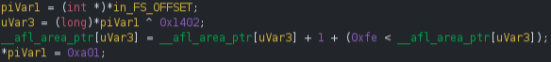
The first noticeable change is that the prev_location variable is no longer global but implemented using thread-local storage, ensuring multi-threaded targets don’t pollute each other’s coverage. By keeping prev_location per-thread, the fuzzer avoids this interference and ensures that coverage information reflects the execution path of each thread independently.
At a higher level, the rest of the logic still follows AFL’s original encoding scheme: the index into the shared coverage map is calculated as
cur_location ^ prev_location, the corresponding counter in the 64 kB bitmap is incremented, and prev_location is updated with the shifted value of the current block
(cur_location = prev_location >> 1). What changes in AFL++ is how the compiler materializes these operations. In the snippet, the right shift has already been applied to the constant at compile time, so instead of seeing a shift instruction we observe the adjusted immediate value directly (0x1402 >> 1 = 0xa01).
The counter update looks cryptic at first glance, but this is nothing more than increment-with-overflow-protection. We can see this better if we peek into the assembly code:
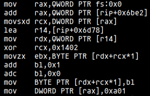
The instructions add bl, 0x1 followed by adc bl, 0 ensure that if the counter at __afl_area_ptr[idx] reaches 255 and wraps, the carry flag forces the value back to 1 instead of 0. In decompiled form this appears as __afl_area_ptr[idx] = __afl_area_ptr[idx] + 1 + (0xfe < __afl_area_ptr[idx]). The effect is that execution frequency remains bounded without losing precision, since a saturated counter at 255 never resets silently.
Finally, the prev_location is updated with the shifted current location, closing the cycle for the next edge calculation. In this case, as noted earlier, the compiler directly materializes the constant 0xa01 instead of performing the shift dynamically.
NATIVE
This mode corresponds to the LLVM’s PCGUARD implementation, thus the name of native.

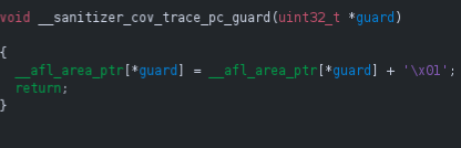
If we open the compiled binary in ghidra, we can observe that a call to the function __sanitizer_cov_trace_pc_guard(uint32_t *guard) is inserted on every edge.
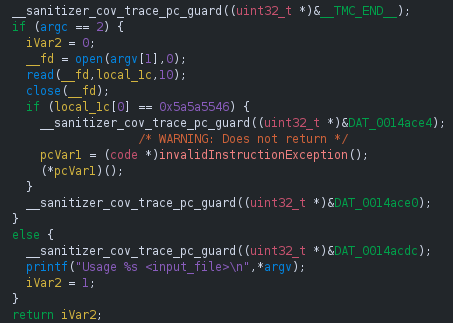
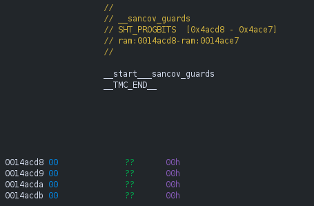
As you may have noticed, each call passes the address of a unique uint32_t guard variable that the compiler emits for every instrumented edge. These guard variables are not placed in the usual .bss or .data segments, but instead collected in a dedicated section named __sancov_guards. At link time, the start and end of this section are exposed through the special symbols __start___sancov_guards and __stop___sancov_guards, so that all guards can be discovered as a contiguous array. If we follow the reference of one of the DAT_* reference, we end up in the __sancov_guards section:
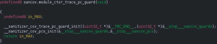
During program startup, a compiler-generated constructor calls __sanitizer_cov_trace_pc_guard_init(__start___sancov_guards, __stop___sancov_guards), which assigns each guard an index into __afl_area_ptr. As stated by the LLVM documentation, each __sanitizer_cov_trace_pc_* function should be defined by the user. AFL++ defines it in the file instrumentation/afl-compiler-rt.o.c.
At runtime, whenever control flows across an instrumented edge, the call to __sanitizer_cov_trace_pc_guard(&guard) is executed. The function reads the guard’s identifier, uses it to record coverage, and may reset it to zero to avoid duplicate reports.
In some configurations, a companion section named __sancov_pcs is also present, containing program counter values for each edge, which can be combined with guard IDs to map runtime coverage information back to specific code locations.
PCGUARD
This mode is an AFL++ implementation of the LLVM PCGUARD described above. It is the default option since commit 5d0bcf. This option is also available by using
afl-clang-fast / afl-clang-fast++.

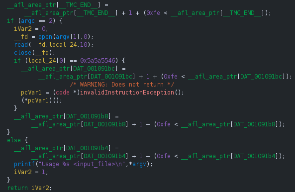
If we open the compiled binary in ghidra, we can observe that calls to the function __sanitizer_cov_trace_pc_guard(uint32_t *guard) have been inlined.
LTO
This mode is very similar to PCGUARD except thta the instrumentation is performed at link time. To do so, the binary is compiled in LTO (Link Time Optimization) mode.
LTO was added in commit 9d686b. Additionally, by default ships with the AUTODICTIONARY feature: while compiling, a dictionary based on string comparisons is automatically generated and put into the target binary.
This option is also available by using afl-clang-lto / afl-clang-lto++.

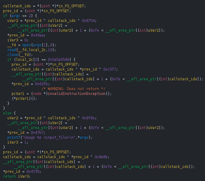
If we open the compiled binary in ghidra, we can observe that the inlined code is a little bit different: the index into __afl_area_ptr is an immediate instead of a variable.
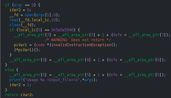
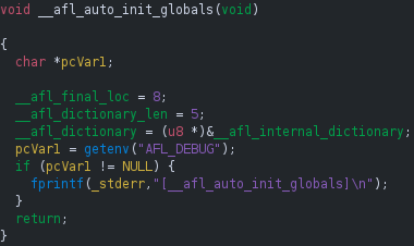
A key distinction of LTO mode is that the mapping of instrumentation sites to the coverage map is resolved at link-time, as we have seen. Because each site’s index into __afl_area_ptr is embedded as an immediate value, a runtime guard-mapping function is not needed. Instead, this mode uses the __afl_auto_init_globals constructor, found in instrumentation/afl-compiler-rt.o.c, to initialize other runtime features that we’ll explore in the next post.
The main differences between PCGUARD and LTO, as pointed out here are:
- 10-25% speed gain compared to llvm_mode
- The compile time, especially for binaries to an instrumented library, can be much (and sometimes much much) longer.
CTX
The next mode was introduced on commit 9ef4b4 and is an LLVM-based implementation of the context sensitive branch coverage.

Here, every function gets a unique ID and, every time when an edge is logged, all the IDs in the callstack are hashed and combined with the edge transition hash. The expression used to collect the coverage is updated as follows:
map[cur_location_ID ^ prev_location_ID >> 1 ^ hash_callstack_IDs] += 1.
If the context sensitive coverage introduces too may collisions and becoming detrimental, the user can choose to use only the called function ID, instead of the entire callstack hash, thus changing the expression again: map[cur_location_ID ^ prev_location_ID >> 1 ^ prev_callee_ID] += 1.
To enable this mode you can set the either the env variable AFL_LLVM_INSTRUMENT to CALLER or AFL_LLVM_CALLER to 1.
NGRAM-x
Finally, the last available mode was introduced on commit 5a74cf and is an LLVM-based implementation of the n-gram branch coverage proposed in the paper “Be Sensitive and Collaborative: Analyzing Impact of Coverage Metrics in Greybox Fuzzing” by Jinghan Wang, et. al.

The number of branches to remember is an option that is specified either in the AFL_LLVM_INSTRUMENT=NGRAM-{value} or the AFL_LLVM_NGRAM_SIZE env variable. The expression used to collect the coverage depends on the value of n:
map[cur_location_ID ^ prev_location[0] >> 1 ^ prev_location[1] >> 1 ^ …] += 1.
Summary
This post lays the groundwork for understanding how AFL++ instruments a program to track code coverage. We reviewed the basics of fuzzing (black-box vs. gray-box) and coverage metrics (edges vs. blocks) to explain the motivation behind AFL++’s design, then analyzed the instrumentation modes, from the original AFL edge hash to modern LLVM-based approaches like PCGUARD and LTO.
In the next post, we’ll dive into the compilation process step by step—how targets are built and instrumented—before moving on to runtime feedback in afl-fuzz and seeing how new execution paths are actually discovered.